Last week I explained a bit about how my prediction model came into being, and how it works. The “flip” component of it, which identifies questionable spreads and presumes a trap is being set, is responsible for the majority of the money the computer bets each week and primarily focuses on favorites. But there’s also a “hedge” component, which bets exclusively on underdogs.
In general, bettors prefer favorites, mainly as a psychological spillover of the fact that favorites win the actual game 66% of the time. But the spread is a powerful equalizer. The Detroit Lions lost all eighteen games last year. They were the worst team in NFL history. They got beat by more than 17 points seven times. They kept the final score within a touchdown only three times. And yet Vegas set the spread at 11 points or greater only seven times during the season. And every single time – every single time – the Lions were able to keep the game close enough to cover it.
In the last twelve years, underdogs have won 51.5% of the games against the spread. So statistically, the underdog is the better side to bet. And the prospect of betting on home dogs has been well-publicized; they have won money 52.2% of the time in the last twelve years. But the last two years have been pretty tough on home dogs; their overall record against the spread is 76-90-3 – a win percentage of just 47.5%. Blanket projections like this are a dangerous way to bet, as are most trends – they’re statistical fluctuations which are just as likely to bounce back (particularly if they are well-known) as they are to uphold their performance.
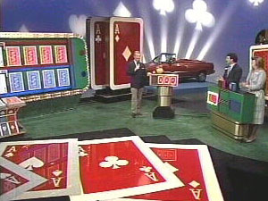
 There’s a statistical phenomenon called “regression to the mean” which refers to the tendency of sequential outcomes to find their way back towards the center of the distribution. The further away from that “center” that any one particular outcome lies, the more likely it is that the following outcome will be closer to the center than the last. The easiest way to envision this is with the classic game show “Card Sharks” (or perhaps the drinking game high-low-red-black). Players would be dealt a card and have to guess whether the next card would be higher or lower. When presented with a low card (for example, a four), most contestants would (wisely) predict that their next card would be higher. Of course, there is no inherent skill involved in this process; it’s simply a matter of luck. And attempting to apply this to football, where skill is very much a factor in determining the outcome of a game, must be done carefully. But luck is also a factor in football games, as well as the tendency of lousy teams to improve and talented teams to deteriorate. And in cases where the spread is perfectly balanced, the underdog has an inherent edge because both of these factors work in its favor.
Each week the computer identifies four or five favorites that pass muster under the “flip” method. Based on the model’s past performance, these favorites should have an above-average chance of winning. Which means that amongst the remaining games, any given underdog has a slightly higher chance than the base of 51.5%. It only takes a small edge to get over the breakeven point – and by taking the games where the computer sees a spread as being set perfectly (less than a 55% confidence level), it’s possible to take advantage of this plus the “regression to the mean” potential. The hedge bets aren’t as powerful – they only hit 53.4% of the time, but they make things more interesting.
The betting scheme I used last year and plan to continue this year is based on a steady growth strategy. Hedge bets are given a weighting of 1. Confidence levels of 85% are given a weighting of 3. Confidence levels of 90% are given a weighting of 8. Confidence levels of 95% or better are given a weighting of 25. Each week, the base amount grows by 1%. For the first week of 2009, the base amount is $0.21. Which means that if ten of the models picked Dallas at a confidence level of between 85% and 90%, the total bet for the game would be $6.24 (0.21 x 3 x 10).
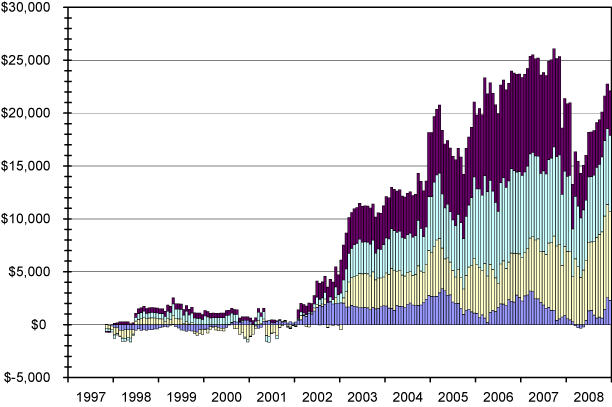
Occasionally, when one of the teams has particularly volatile statistics, it’s possible for the “flip” scheme and the “hedge” scheme to come into conflict. In this case, the computer will side with whichever scheme dominates (after weighting) and subtract the weaker side’s component from the overall bet. Sometimes the two schemes agree, in which case the total bet is the sum of the two. The graph below shows the performance after eleven years, based on a starting value similar to what I’ll be starting with this year.
It would have taken quite a bit of faith to stick with the computer during the lean years of 2000 to 2001. But the boom years between 2002 and 2006 more than made up for it. The model took a bit hit at the end of 2007 and the beginning of 2008, but with sufficient faith it’s shown a pretty spectacular return. This progression is based on 10% juice (and includes pushes), but I make an effort to take advantage of nickel (5%) juice whenever I can – it makes a pretty significant difference over time.
Stop by next week – I’ll have my picks for the first week of the season.


Comments